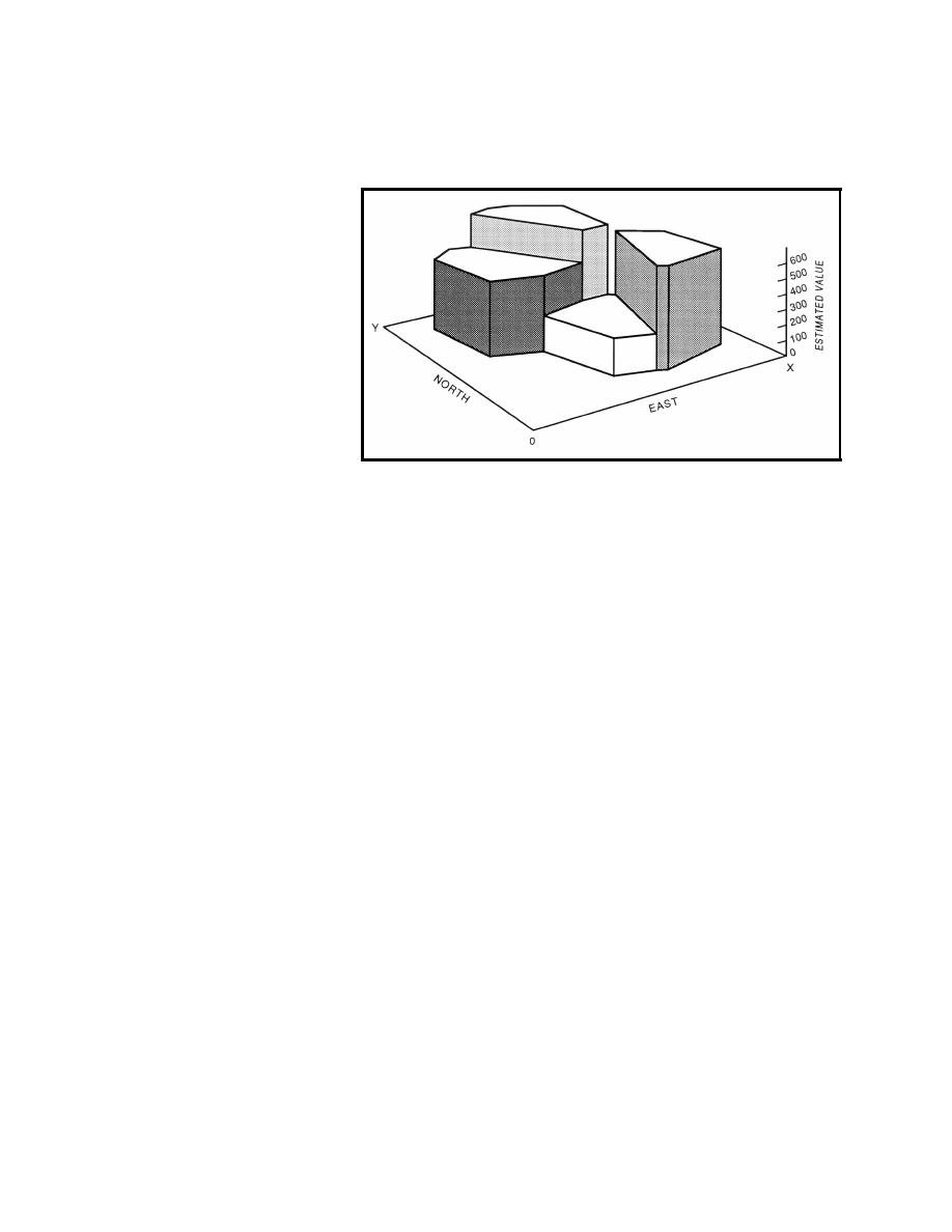
Figure 5. Polygonal point estimating method (adapted from Isaaks and Srivastava 1989)

ERDC TN-DOER-C15

July 2000

adaptations of inverse distance declustering methods. In the polygonal method, the sample value

closest to the point being estimating is selected as the estimate. This value holds throughout the

polygon of influence constructed around the estimated point. This method results in discontinuous

parameter distributions over the

area of interest (Figure 5).

The method of triangulation

eliminates these discontinuities

by fitting a plane through three

samples surrounding the point

to be estimated. An equation of

the plane is developed that can

be solved for the estimated pa-

rameter value at any point

within the triangle by substitut-

ing the coordinates of the point.

Alternatively, weighting fac- Figure 5. Polygonal point estimating method (adapted from Isaaks

tors can also be derived using

and Srivastava 1989)

triangulation. Inverse distance

methods apply a weighting factor to nearby samples that is inversely proportional to the distance

of the data point from the point being estimated. Some power p of the distance may also be used;

small values of p decrease the difference in the weighting factors and larger values of p increase the

difference. These methods are more fully described in Isaaks and Srivastava (1989).

Selection of nearby samples used as the basis for point estimation is also an important step in the

estimating process, and may also be a consideration in location of initial sampling points. Isaaks

and Srivastava (1989) refer to areas containing relevant samples as "search neighborhoods." Within

the search neighborhood there must be a sufficient number of nearby samples, but not too many or

redundant samples. The relevance of samples falling within the search neighborhood should also

be considered. The number of samples to include is particularly important to inverse distance and

kriging. The number of samples included using geometric estimating techniques is self-determin-

ing, based upon the orientation of the samples.

Normally, all available samples within the defined search neighborhood are used in estimation.

Typically, an ellipse is centered on the point being estimated, with the long axis oriented in the

direction of greatest continuity of the sample values (Isaaks and Srivastava 1989). In a CDF, this

would likely be horizontally across the cell, perpendicular to the direction of flow. The length to

width of the ellipse is determined by judgment, based on the degree of anisotropy evidenced in the

available data.

Alternatively, all samples within a specified distance of the point to be estimated might be used.

For regularly gridded data, the search neighborhood should be at least large enough to include the

four nearest samples. In practice, a minimum of 12 samples is typical (Isaaks and Srivastava 1989).

The search neighborhood for irregularly gridded data should be just larger than the average spacing

between the sample data, estimated as follows (Isaaks and Srivastava 1989):